The connection between the Laplace and Fourier transforms
Table of contents
This is a short article discussing how the Laplace and Fourier transforms, two important tools in engineering mathematics, are related.
The Fourier transform
The Fourier transform of some function \(x(t)\) is defined as:
\[X(\omega) = \int_{-\infty}^{\infty} x(t) e^{-i\omega t} \, dt\]Suppose we have a function \(x(t) = e^{-k t} \sin(\Omega t)\). Then, its Fourier transform is found to be:
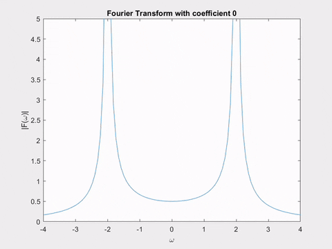
\[X(\omega) = \frac{\Omega}{\omega^2 + \Omega^2}\]Notice that the function diverges at the points \(\omega = \pm \Omega\). Therefore, the Fourier transform tells us that the function has a sinusoid somewhere with angular frequency \(\Omega\) (which we know, of course, because we knew the function already).
The Fourier transform tells us the angular frequencies \(\omega_i\) of all the sinusoids present in some function \(x(t)\).
Below is a plot of the magnitude of the Fourier transform of \(x(t) = e^{-0.5 t} sin(2t)\), produced using MATLAB.

The Laplace transform
The Laplace transform of a function \(x(t)\) is defined as:
\[\mathcal{L}\{x(t)\} = \int_{0}^{\infty} x(t) e^{-s t} \, dt\]where \(s\) is a complex number, such that:
\[s = \alpha + i \omega\]Substituting this form of \(s\) into the Laplace transform formula, we obtain:
\[\mathcal{L}\{x(t)\} = \int_{0}^{\infty} x(t) e^{-i \omega t} e^{- \alpha t} \, dt\]Notice that this is now almost identical to the formula we had for the Fourier transform of \(x(t)\)! Using \(x(t) = e^{-k t} \sin(\Omega t)\), as we had before, we can evaluate the integral, and find that:
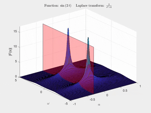
\[\mathcal{L}\{x(t)\} = \frac{\Omega}{(k + \alpha + i \omega)^2 + \Omega^2}\]To visualise the Laplace transform, we can use a 3D plot, with the first two axes corresponding to \(\alpha = \text{Re}(s)\) and \(\omega = \text{Im}(s)\), and the height of the plot set to \(\|\mathcal{L}\{x(t)\}\| = \|F(s)\|\) (another notation for the Laplace transform). Note that we’re plotting the magnitude of the Laplace transform only here. For the function \(x(t) = e^{-0.5 t} sin(2t)\), the Laplace transform looks like this:

By analysing the denominator of this function, we can see the poles will occur at the coordinates \((\alpha, \omega) = (-0.5, \pm 2)\). Not only are we given information about the sinusoids present, but we also now know the coefficient of the exponential pre-factor, from the value of \(\alpha\) at the poles!
The poles of the Laplace transform \(\mathcal{L}\{x(t)\}\) tell us about the exponentials and sinusoids present in a function \(x(t)\).
How are the two transforms related?
When you compute the 2D plot of the Fourier transform of a function, you are actually taking a 2D slice of the Laplace transform of that function. Let’s return to the form of the Laplace transform we had earlier:
\[\mathcal{L}\{x(t)\} = \int_{0}^{\infty} x(t) e^{-i \omega t} e^{- \alpha t} \, dt\]If we set \(\alpha\) to zero, this just collapses to \(X(\omega)\), the Fourier transform of \(x(t)\). So the Fourier transform of a function is just the Laplace transform for \(\alpha = 0\), where \(s = \alpha + i \omega\).
Actually, all the Laplace transform is doing is repeatedly finding the Fourier transform of a modified function \(x(t, \alpha) = x(t) e^{-\alpha t}\). Each time, we adjust \(\alpha\) by a small amount, then recompute the Fourier transform and plot its magnitude! I’m going to show two animations that demonstrate this.
The first animation shows the Fourier transform of \(e^{-\alpha t} \sin(2t)\), for varying \(\alpha\). Can you notice the similarity between the changing shape of the Fourier transform, and the shape of the Laplace transform poles we saw earlier?
The second animation shows a plane in the Laplace transform of \(sin(2t)\). As we move it, notice the shape of the curve traced out by the intersection of the plane with the Laplace transform’s surface - it’s exactly the Fourier transform we just saw in the animation!
Key results
- The Laplace transform is a generalisation of the Fourier transform.
- The Fourier transform is a special case of the Laplace Transform for when \(s\) is purely imaginary, i.e. \(\alpha = 0\).
- We can interpret the Fourier transform as a 2D slice of the Laplace transform in the plane \(\text{Re}(s) = 0\).